DBSCAN(Density-Based Spatial Clustering of Applications with Noise)是一種密度聚類算法,用於將數據點劃分為多個集群,同時可以識別和排除噪音點。該算法基於以下概念:
- 核心點(Core Points):對於給定的半徑 $\varepsilon$ (epsilon)內至少包含 $min_samples$ 個數據點的點被視為核心點。
- 邊界點(Border Points):如果一個點不是核心點,但位於某個核心點的 $\varepsilon$ 鄰域內,則它被視為邊界點。
- 噪音點(Noise Points):不是核心點也不是邊界點的數據點被視為噪音點。
DBSCAN算法運行步驟如下:
- 選擇一個未訪問的數據點作為起始點,檢查其 $\varepsilon$ 鄰域內的點數量:
- 如果該點是核心點,則將其與其 $\varepsilon$ 鄰域內的所有點標記為同一個集群。
- 如果該點是邊界點,則將其標記為集群的一部分。
- 對於已訪問的核心點,擴展集群並標記所有可達的點。
- 重複步驟1和步驟2,直到所有點都被訪問過。
DBSCAN的主要優勢是:
- 能夠在集群之間具有不同的形狀和大小。
- 能夠識別和排除噪音點。
- 不需要事先指定要劃分的集群數量。
總的來說,DBSCAN是一種強大的聚類算法,特別適用於處理具有不同密度和形狀的數據集。
import numpy as np
import matplotlib.pyplot as mpl
from scipy.spatial import distance
from sklearn.cluster import DBSCAN
# Creating data
c1 = np.random.randn(100, 2) + 5
c2 = np.random.randn(50, 2)
# Creating a uniformly distributed background
u1 = np.random.uniform(low=-10, high=10, size=100)
u2 = np.random.uniform(low=-10, high=10, size=100)
c3 = np.column_stack([u1, u2])
# Pooling all the data into one 150 x 2 array
data = np.vstack([c1, c2, c3])
# Calculating the cluster with DBSCAN function.
# db.labels_ is an array with identifiers to the
# different clusters in the data.
#db = DBSCAN().fit(data, eps=0.95, min_samples=10)
db = DBSCAN().fit(data)
labels = db.labels_
# Retrieving coordinates for points in each
# identified core. There are two clusters
# denoted as 0 and 1 and the noise is denoted
# as -1. Here we split the data based on which
# component they belong to.
dbc1 = data[labels == 0]
dbc2 = data[labels == 1]
noise = data[labels == -1]
# Setting up plot details
x1, x2 = -12, 12
y1, y2 = -12, 12
fig = mpl.figure()
fig.subplots_adjust(hspace=0.1, wspace=0.1)
ax1 = fig.add_subplot(121, aspect='equal')
ax1.scatter(c1[:,0], c1[:,1], lw=0.5, color='#00CC00')
ax1.scatter(c2[:,0], c2[:,1], lw=0.5, color='#028E9B')
ax1.scatter(c3[:,0], c3[:,1], lw=0.5, color='#FF7800')
ax1.xaxis.set_visible(False)
ax1.yaxis.set_visible(False)
ax1.set_xlim(x1, x2)
ax1.set_ylim(y1, y2)
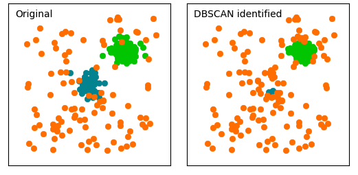
ax1.text(-11, 10, 'Original')
ax2 = fig.add_subplot(122, aspect='equal')
ax2.scatter(dbc1[:,0], dbc1[:,1], lw=0.5, color='#00CC00')
ax2.scatter(dbc2[:,0], dbc2[:,1], lw=0.5, color='#028E9B')
ax2.scatter(noise[:,0], noise[:,1], lw=0.5, color='#FF7800')
ax2.xaxis.set_visible(False)
ax2.yaxis.set_visible(False)
ax2.set_xlim(x1, x2)
ax2.set_ylim(y1, y2)
ax2.text(-11, 10, 'DBSCAN identified')