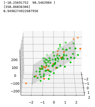
首先,使用make_regression函數生成了一些合成數據,然後將數據分成訓練集和測試集。接著創建了LinearRegression模型的實例,並使用訓練集對模型進行訓練。訓練完成後,打印出了模型的係數和對新數據的預測結果。最後,通過可視化將訓練集和測試集的散點圖以及線性回歸的平面呈現出來。
import numpy as np
import matplotlib.pyplot as mpl
from mpl_toolkits.mplot3d import Axes3D
from sklearn import linear_model
from sklearn.datasets import make_regression

# Generating synthetic data for training and testing
X, y = make_regression(n_samples=100, n_features=2, n_informative=1, random_state=0, noise=50)

# X and y are values for 3D space. We first need to train
# the machine, so we split X and y into X_train, X_test,
# y_train, and y_test. The *_train data will be given to the
# model to train it.
X_train, X_test = X[:80], X[-20:]
y_train, y_test = y[:80], y[-20:]

# Creating instance of model
regr = linear_model.LinearRegression()

# Training the model
regr.fit(X_train, y_train)

# Printing the coefficients
print(regr.coef_)
# [-10.25691752 90.5463984 ]
# Predicting y-value based on training
X1 = np.array([1.2, 4])
print(regr.predict([X1]))
# 350.860363861
# With the *_test data we can see how the result matches
# the data the model was trained with.
# It should be a good match as the *_train and *_test
# data come from the same sample. Output: 1 is perfect
# prediction and anything lower is worse.
print(regr.score(X_test, y_test))
# 0.949827492261

fig = mpl.figure(figsize=(8, 5))
ax = fig.add_subplot(111, projection='3d')
ax.view_init(elev=20, azim=0)
# ax = Axes3D(fig)
# Data
ax.scatter(X_train[:,0], X_train[:,1], y_train, facecolor='#00CC00')
ax.scatter(X_test[:,0], X_test[:,1], y_test, facecolor='#FF7800')

# Function with coefficient variables
coef = regr.coef_
line = lambda x1, x2: coef[0] * x1 + coef[1] * x2
grid_x1, grid_x2 = np.mgrid[-2:2:10j, -2:2:10j]
ax.plot_surface(grid_x1, grid_x2, line(grid_x1, grid_x2), alpha=0.1, color='k')
ax.xaxis.set_visible(False)
ax.yaxis.set_visible(False)
ax.zaxis.set_visible(False)