內插法是一種數學方法,用於在已知數據點之間估算未知點的值。在內插中,我們假設數據點之間的關係是連續且光滑的,並使用這種關係來預測未知位置的數值。
具體來說,當我們有一組離散的數據點,但我們想要在這些點之間的某個位置獲得更多的數據時,我們就可以使用內插法。它通常用於曲線擬合和數據補充的情況下,幫助我們理解數據的行為、預測趨勢或填補缺失的數據。
在內插中,我們根據已知的數據點來建立一個函數或曲線,該函數或曲線在這些點上通過已知的數據點,並且在這些點之間是連續且光滑的。然後,我們使用這個函數或曲線來估算我們感興趣的位置的值。
內插法有很多種類,包括線性內插、多項式內插、樣條內插等。選擇適當的內插方法取決於數據的特性和應用的需求
SciPy提供了十幾種不同的插值函數,從簡單的單變量情況到複雜的多變量情況。當樣本數據可能由一個獨立變量引導時,使用單變量插值,而多變量插值則假設存在多個獨立變量。 內插法有兩種基本方法:(1)對整個數據集擬合一個函數或(2)用多個函數擬合數據集的不同部分,其中每個函數的連接部分平滑地連接在一起。
import numpy as np
import matplotlib.pyplot as plt
from scipy.interpolate import interp1d
#產生已知數據
x = np.linspace(0, 10 * np.pi, 20)
y = np.cos(x)
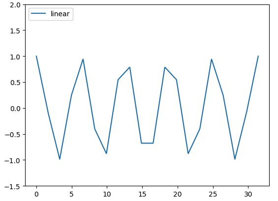
#使用線性內插(擬合),得到f1線性函式
f1 = interp1d(x, y, kind='linear')
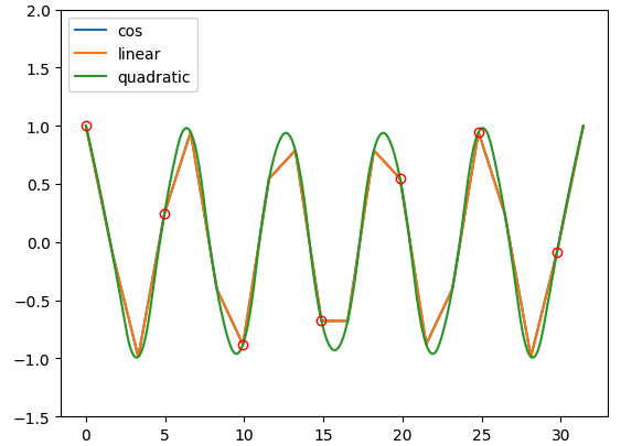
#使用二次內插(擬合),得到fq二次函式
fq = interp1d(x, y, kind='quadratic')
#尋找兩個函式間的交點,初始猜測值(x點座標)
result = findIntersection(f1, fq, [0, 5, 10, 15, 20, 25, 30])
xint = np.linspace(x.min(), x.max(), 1000)
plt.ylim(-1.5, 2)
plt.plot(x, y, label='cos')
plt.plot(xint, f1(xint), label='linear')
plt.plot(xint, fq(xint), label='quadratic')
plt.plot(result, fq(result), 'ro', markerfacecolor='none')
plt.legend(loc='upper left')
plt.show()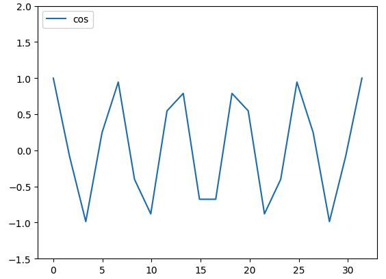
我們接下來使用一個複雜的邏輯來產生數據,再使用Scipy的內插(擬合)函式來找出合適的資料模型函式。
import numpy as np
import matplotlib.pyplot as plt
from scipy.interpolate import UnivariateSpline
from scipy.optimize import fsolve

#尋找兩函式的交點
def findIntersection(func1, func2, sample, x0):
    return fsolve(lambda x: func1(x) - func2(x, sample), x0)

sample = 30

#更複雜的函式
x = np.linspace(1, 10 * np.pi, sample)
def func(x, sample):
    return np.cos(x) + np.log10(x) + np.random.randn(sample) / 10
y = func(x, sample)

#一元二次樣條函式
f = UnivariateSpline(x, y, s=1)

#尋找兩函式的交點
result = findIntersection(f, func, 6, [5, 10, 15, 20, 25, 30])


xint = np.linspace(x.min(), x.max(), 1000)
plt.plot(x, y, label='origin')
plt.plot(xint, f(xint), label='UnivariateSpline')
plt.plot(result, f(result), 'ro', markerfacecolor='none')
plt.legend()
plt.show()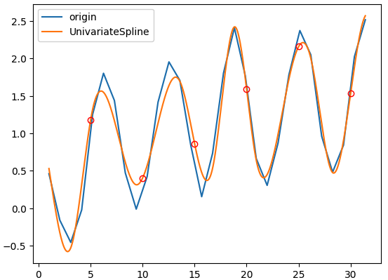
import numpy as np
from scipy.interpolate import griddata
# Defining a function
ripple = lambda x, y: np.sqrt(x**2 + y**2)+np.sin(x**2 + y**2)
# Generating gridded data. The complex number defines
# how many steps the grid data should have. Without the
# complex number mgrid would only create a grid data structure # with 5 steps.
grid_x, grid_y = np.mgrid[0:5:1000j, 0:5:1000j]
# Generating sample that interpolation function will see
xy = np.random.rand(1000, 2)
sample = ripple(xy[:,0] * 5 , xy[:,1] * 5)
# Interpolating data with a cubic
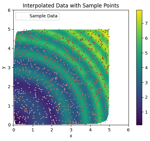
# griddata 是 SciPy 中的一個函數,用於在非結構化的數據點集上進行插值。當你有一組數據點,但## #它們不是均勻分佈在網格上時,你可以使用 griddata 將這些數據點的值插值到指定的網格上,以獲得在整個網格上的連續數值。
# 具體來說,griddata 函數接受三個主要的參數:
# points:數據點的坐標。
# values:對應於每個數據點的值。
# grid:指定用於插值的目標網格。
# griddata 根據給定的數據點和對應的值,在目標網格上進行插值,並返回整個網格上的插值結果。插值方法可以通過 method 參數指定,包括線性插值、最近鄰插值和立方插值等。
grid_z0 = griddata(xy * 5, sample, (grid_x, grid_y), method='cubic')
# 繪製內插後的圖像
plt.ylim(0, 6)
plt.xlim(0, 6)
plt.imshow(grid_z0, extent=(0, 5, 0, 5), origin='lower', cmap='viridis')
# 添加色標
plt.colorbar()
# 繪製樣本數據的散點圖
plt.scatter(xy[:, 0] * 5, xy[:, 1] * 5, c=sample, cmap='Reds', label='Sample Data', s=1)
# 添加標籤和標題
plt.xlabel('x')
plt.ylabel('y')
plt.title('Interpolated Data with Sample Points')
plt.legend(loc='upper left')
# 顯示圖像
plt.show()